You can change cell colour in an Excel spreadsheet automatically by increasing or decreasing the number value in the cell. Through this process, one can easily find out the highest or lowest value. To do so, you can follow 2 methods explained in this article.
Table of Contents
Change Cell Color Based on Value in Excel
Method 1:
Enter different number values in each cell of a range.
Select the range of cells that contains number values
As soon you select the number values in a range of cells, a quick analysis tool’s icon will be presented at the bottom right.
Click the icon to expand its options.
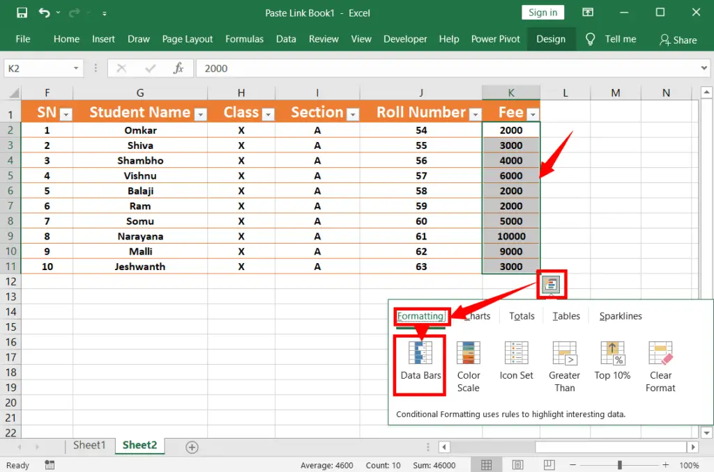
Under “Formatting”, select “Data bars” to fill in based on the cell value.

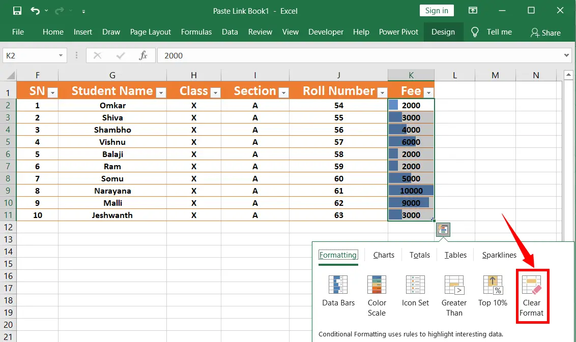
If you want to remove the cell background colour, click “Clear format”.
Method 2:
Enter different number values in each cell of a range.
Select the range of cells that contains number values
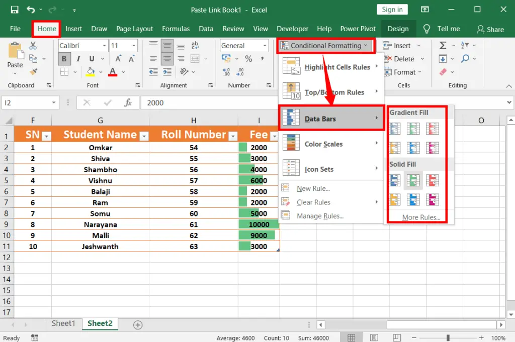
Click “Conditional formatting” on the “Home” tab to expand its menu
Now hover over “Data bars”, then select “Gradient fill” or “Solid fill” based upon your recommendation.
Changing the cell colour in an Excel spreadsheet depends on the number value. It is difficult to read each value one by one and find the value we want. Hence through this process, you can easily find out the highest or lowest value very.
For example in class 10th those who got 90+ marks and those who got less than 35 should be identified easily then what will you do? Not only the marks but also their attendance can be easily identified through this process.
Is it possible to add the cell colour based on a value in Excel?
Yes
How to identify the highest or lowest value in excel
To find such value in Excel, you must use the Data Bars in Conditional Formatting.
How to Apply Conditional Formatting in Excel?
Go to “Conditional Formatting” in the “Home” tab, set rules based on values, and choose colors for formatting.
Handling Multiple Rules for One Cell?
Excel applies the first matching rule, so arrange rule priorities in the Conditional Formatting Rules Manager.
Can I create custom color scales for conditional formatting?
Yes, Excel allows you to create custom color scales with specific colors and criteria to highlight values in a way that best suits your data analysis needs.