
In Microsoft Excel, Freeze panes helps us to keep portion of the selected rows, columns, or both visible when scrolling the spreadsheet up or down, or left or right.
This feature is particularly helpful when you need to view or work with a large amount of off-screen data, based on the column header or row header, by scrolling.
In this article, we will look into the concept of freeze panes to boost our work speed and save a significant amount of time compared to manual work.
Table of Contents
For example, when the data in the sheet is not fully visible or when you are working with the current data and scrolling downwards or to the right, a portion of the data along with the row header or column header gets hidden on the screen.
Thus, in order to enter or read the data in a worksheet by scrolling horizontally or vertically based on the row and column header, it is necessary to freeze them. This ensures that the row header and column header remain visible and don’t disappear from view.
Benefits of Using Freeze Panes
Freeze panes offers several advantages to Excel users:
- Enhanced Data Analysis: By freezing key rows or columns, you can compare data more efficiently and maintain context while scrolling through extensive datasets.
- Efficient Navigation: Freeze panes enables easy navigation within large spreadsheets, as important information remains visible at all times.
- Improved Presentation: When presenting data or sharing spreadsheets with others, freezing panes ensures that important information is always visible, eliminating the need for scrolling or excessive manual adjustments.
Now that we’ve covered the basics of freeze panes and their benefits, let’s look at how to do it in Excel.
How To Freeze Panes in MS Excel
After entering the data along with the column headings and the row headings start reading descriptive contents or short contents by switching the tabs below.
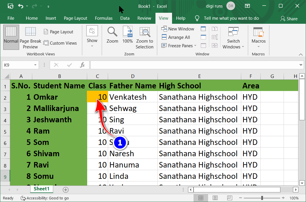
- Click the common cell (orange coloured cell as in the screenshot below) which is underneath the row header and immediate right of the column header as given in the 1st step of the screenshot below
(This is the first step to freezing the row header and column header in the green area).
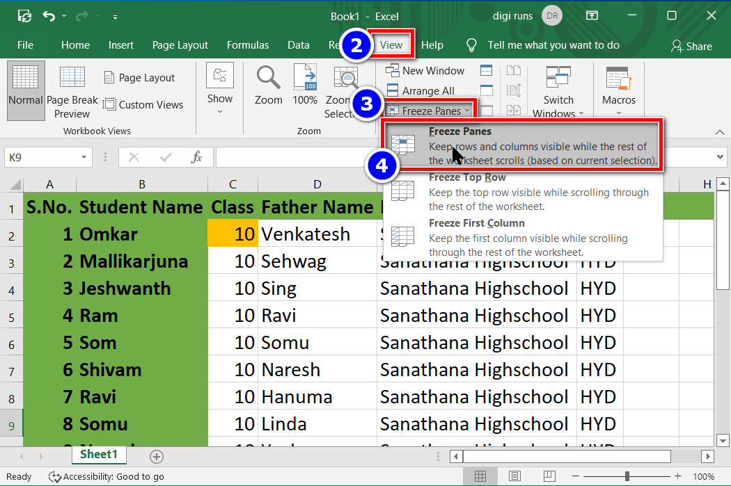
- Next, navigate to the “View” tab
- Click on “Freeze Panes.”
- Afterward, select the option to freeze the same.
- Click on the cell that is commonly shared (indicated by an orange-colored cell, as shown in the screenshot) located directly below the row header and immediately to the right of the column header.
- Next, go to the “View” tab and click on “Freeze Panes.” Then, once again, select the same option underneath it to freeze both rows and columns in Excel.
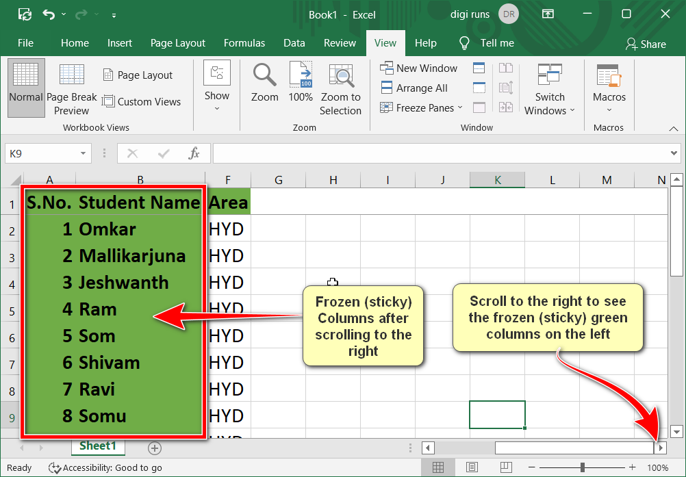
- Now, as shown in the screenshot below, the column and row headers will be frozen.
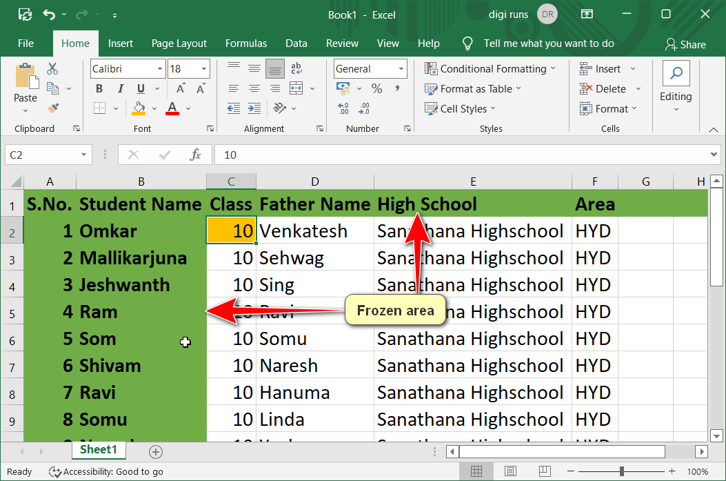
- Now, scroll to the right and then scroll back to the left to see the frozen columns, as instructed in the screenshot below.
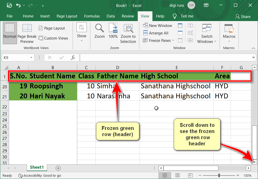
- Similarly, scroll down and then scroll back up to observe the frozen row header, as indicated in the screenshot below.
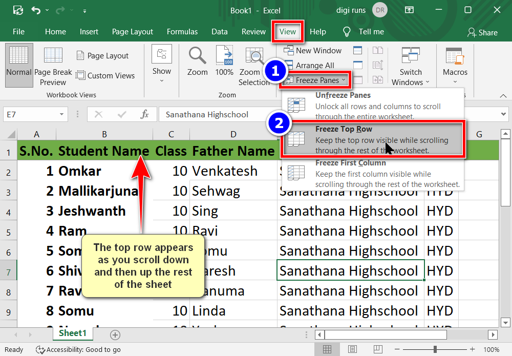
To lock the top row of a worksheet while the rest of the worksheet scrolls, follow the steps below:
- Click on “Freeze Panes“.
- Then, click on “Freeze Top Row“.
- Now, scroll the page left and right to observe the frozen area of the worksheet.
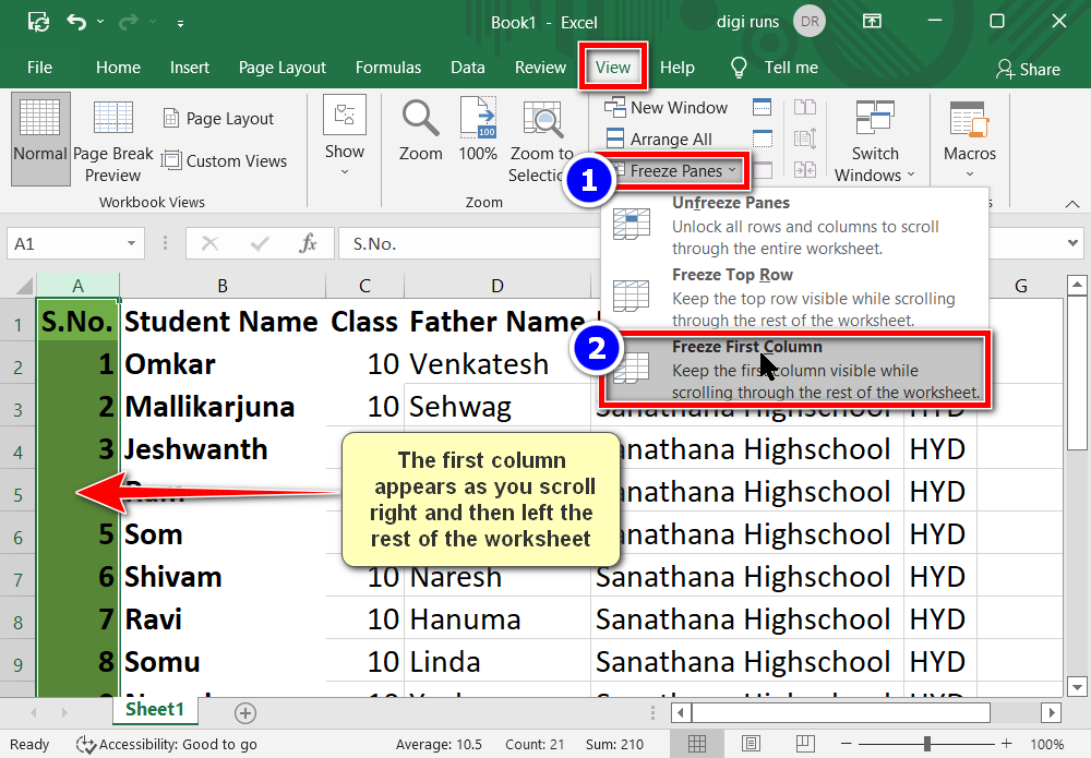
To freeze or lock the first column of a worksheet while the rest of the worksheet scrolls, follow these steps:
- To stick only the first column while scrolling the rest of the screen, click freeae panes
- Next, select “Freeze First Column”. Now, scroll the page to view the frozen area of the worksheet.
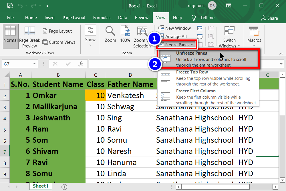
Unfreeze the Panes in Excel
- After freezing the upper part, left part, or both parts of the rows and columns (such as the left column or the first row) in a sheet, click on click on “Unfreeze Panes” on the “View” tab in Excel to remove the frozen panes.
Microsoft Excel’s freeze panes feature is considered one of the most valuable tools for managing and processing large datasets and handling complex tasks within an Excel spreadsheet.
By freezing panes, you can substantially improve your workflow and enhance productivity, regardless of whether you’re working on financial models, data entry, or any other Excel operation.
Video Tutorial
Can we freeze multiple panes in excel
No. Unfortunately, we don’t have such an option.
How to freeze 2 rows in excel?
Unfortunately, we don’t have such an option.
Do we have a freeze panes shortcut in excel?
No, we don’t have such a shortcut yet.
How do I freeze the top row in Excel?
To freeze the top row, select the row below it, go to the “View” tab, and click “Freeze Panes” > “Freeze Top Row.”
How do I unfreeze rows or columns in Excel?
To unfreeze rows or columns, go to “View” > “Freeze Panes” > “Unfreeze Panes.”
What’s the benefit of using Freeze Panes in Excel?
Freeze Panes helps maintain context when scrolling through large datasets, ensuring important headers or labels remain visible as you navigate the spreadsheet.